OLTP vs. OLAP

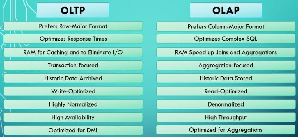
I believe that any discussion on Consistency needs to start from a clear understanding of OLTP and OLAP systems. The below infographic gives a quick comparison snapshot.

Online Transaction Processing (OLTP)

OLTP or Online Transaction Processing is a transaction-focused database category. It is usually found as the first layer of a database that is directly connected to an application layer. 

Transactions that are performed on the application layer are recorded in the OLTP database. Since there are a huge number of transactions that happen in the modern application layer, the priority in designing an OLTP database is in-line with the ability in rapid processing.

The below features are typical an OLTP layer:

• Should be able to handle a large number of insertions, updates and deletions. 
• Should have high availability (24/7/365). Downtimes are costly as it will directly affect end users.
• Rapid response is vital. Hence, one of the key performance parameters is response time. Ideally, this should be in milliseconds.
• Data integrity should be ensured. All users should be able to view and access the same data.
• Very old data is archived. The table sizes are maintained within an optimum size. This helps to avoid processing large tables and helps boost performance.
• The RAM is primarily used to boost caching and eliminate I/O operations for recent transactions.
• Row-major storage format is typically preferred. This is for the purposes of improving the performance of DML operations.
• Indexes can be used to boost performance of record retrieval. This helps to retrieve records faster by enabling faster searches.
• As a thumb rule, OLTP databases are highly normalized to ensure data integrity and avoid anomalies. This saves space at the cost of performance during join operations (since we will have to perform joins to get data from the normalized tables).

Online Analytical Processing (OLAP)

OLAP or Online Analytical Processing systems focus on performing multi-dimensional analysis at high speeds on large volumes of data. This is the typical Data Warehouse or Data Mart database.

It typically acts as the centralized data store for analytical purposes. The OLTP layer feeds into the OLAP layer. OLAP is usually the next major layer of the database where the data is organized and optimized through Data Warehousing techniques. The data gets from the OLTP to OLAP layer via an ETL process.

The below features are typical an OLAP layer:

• Complex queries are run on the OLAP to derive analytic insights. 
• Should be fast when performing aggregate calculations. The primary focus here is throughput. A large number of records should be processed in a short amount of time.
• Infrequent write and frequent read operations. Thus, it should be read-optimized.
• Historic data is stored in an aggregated or transformed form. 
• The RAM is used to speed up joins and aggregations for bulk operations.
• Column-major format is typically preferred. This is to help with optimizing the read operations on column-based analytics.
• Partitions along specific dimensions are used to optimize the performance of the read operations that perform analytic operations along those dimensions.
• As a thumb rule, OLAP databases are denormalized to aid join performance. This boosts performance of read operations at the cost of space (since redundant data is stored in the tables).

Consistency in RDBMS vs. NoSQL

Relational Databases

RDBMS or Relational Database Management System is the old workhorse of database technology. It was the pioneering concept in modern organized data storage.

RDBMS has the following features:

• Data in RDBMS has high data integrity. Every user views the same data.
• There is no partition tolerance for the RDBMS system. As such, they scale vertically.
• RDBMS is the legacy technology. It is time-tested and is used by almost all organizations in some form.
• Scalability and performance are frequent issues with RDBMS once the size of the database crosses a certain threshold.
• It has a fixed schema and structure. Once defined, it is very difficult to impossible to change it.
• Data is stored within tables and schemas.

NoSQL

NoSQL or Not only SQL is the new kid in the block. Its features provide much needed answers for designing distributed databases.

NoSQL systems have the following features:

• Prioritizes availability over consistency (more on this later). So all users may not see the same version of the data.
• Highly scalable with partition tolerance. It can handle huge amounts of data.
• Flexible schema and structure. It is dynamic in nature and can be changed as the development process advances. 
• Data is stored in the form of documents like JSON format.

ACID Semantics

ACID is an acronym that refers to the set of 4 key properties that define a transaction: Atomicity, Consistency, Isolation, and Durability. If a database operation has these ACID properties, it can be called an ACID transaction. The data storage systems that apply these operations are called transactional systems. 

ACID transactions guarantee that each read, write, or modification of a table has the following properties:

• Atomicity – Every transaction is treated as an individual unit. Either the entire statement is executed or none of it is. This property maintains data integrity.
• Consistency – All transactions in the database only make changes to tables in predefined and predictable ways. 
• Isolation – Every user accessing the database is isolated from each other so that their concurrent transactions don’t interfere with each other. 
• Durability – All changes to the database are saved on permanent storage and will not disappear in the event of a system failure.

ACID is mostly used in non-distributed systems. A typical example is an OLTP system connected to an application layer. 

Unless absolutely necessary, ACID is not implemented in large-scale systems. This is because doing so can make the system slower and overcoming that slowness requires very high computational power. This can quickly run up the figures in an expense account (which is something most corporations dislike).

CAP Theorem

The CAP Theorem is a theory which says that during a network failure in a distributed system, it is possible to either ensure availability or consistency of the system – not both.

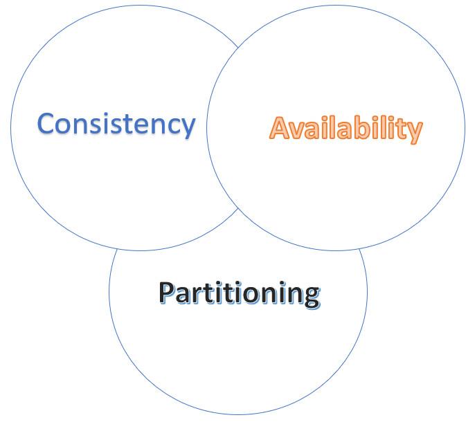
The components of CAP Theorem are as below:

• Consistency – All reads get the most recent writes or an error.
• Availability – All reads get data but need not be the most recent.
• Partition Tolerance – The distributed system continues to operate despite network failures. It might be through dropped partitions, slow connections, etc.

The trade-off between consistency and availability occurs because one comes from the cost of another.

Just imagine a scenario in which we design a distributed system that has high consistency and partition tolerance. In this design, the same data will be stored on multiple servers. When we make an update to a record in one of the partitions (let’s call it the primary node), the change needs to be reflected in its copy on the other partitions (let’s call them secondary nodes). 

Suppose a read request comes in at one of the secondary nodes BEFORE the change from the primary node has reflected in it. When we prioritize consistency in our design, the read operation will have to wait until the change in the primary node is reflected in the secondary nodes. In this way, the users will be able to read the results of the latest write operation on a particular record.

On the other hand, if we had prioritized availability over consistency, the read operation would have been able to fetch the current value in the secondary node instead of waiting till the write operation in the primary node is reflected in the secondary nodes. In this way, the users will be able to read an available result; just not necessarily the latest change.

Consistency in ACID vs. CAP

The C in ACID refers to application-defined semantics. When we say Consistency in a system that ensures ACID, it means that the processing of a transaction does not violate referential integrity constraint rules or such type of application defined rules. 

What is expected of the term Consistency in ACID is that any operation performed on a database should make changes to the data in predefined and predictable ways.

Whereas C of CAP refers to the rules related to making a concurrent, distributed system appear like a single-threaded, centralized system. A read operation of a certain record on any node in this system should fetch the latest update made to that record no matter which node processed it. 

The expectation from the term Consistency in CAP theorem is that in the event that there are multiple copies of the same data distributed across different servers/nodes, every user accessing any node to look for that data should get the same version of data at a given point in time. 

BASE State

As we saw in the earlier section, ACID is quite stringent with regards to its expectations on data integrity. For many applications, it is far too stringent than what the actual use case of the business requires.

BASE stands for  Basically Available Soft-State Eventually Consistent Systems. I know. The acronym is slightly off the mark, right? 🙂

Let’s break this down:

• Basically Available – The database is available and working most of the time. These systems are typically large-scale and stress on Availability.
• Soft-State – Different nodes don’t have to be mutually consistent w.r.t the same data. Thus, we cannot expect (nor it may be necessary) to have all users access the same version of data at a given point in time.
• Eventually Consistent – Following soft-state, we expect only a loose type of consistency in these systems. Thus, all nodes that have the same data may ‘eventually’ sync up. 

BASE is typically used for large-scale data where implementing ACID is not worth the implementation cost and maintaining Consistency is not really important to the business case. Typical examples are highly available systems like sensor data collection.

Sequential Consistency

In Sequential Consistency, every write in the distributed system must be globally ordered.

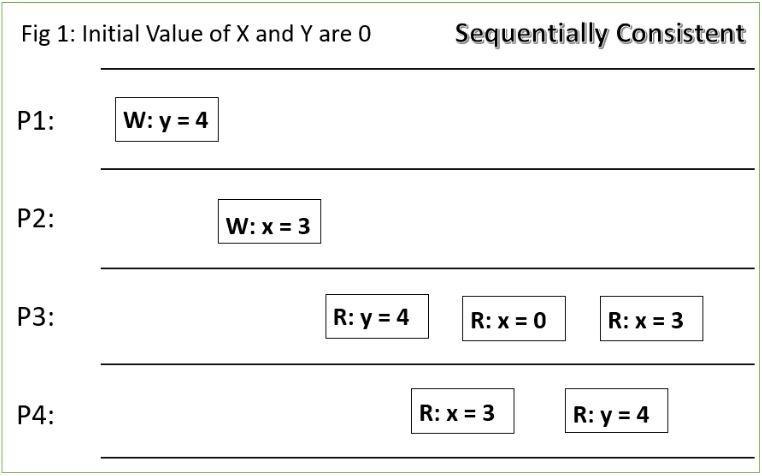
Consider the above figure (Fig 1). P1, P2, P3 and P4 are threads or nodes in a distributed system. W means Write and R means Read. Towards the right indicates chronological sequence. The variables x and y have initial values as 0.

In Fig 1, thread P1 writes y = 4. At a later point in time, the thread P2 writes x = 3. At a point further in time, thread P3 reads the value of y as 3, then reads x as 0 and then reads x as 3. Around this time, thread P4 reads x as 3 and then y as 4.

Here, P4 decides the consistency level. We know that chronologically, the write y = 4 happened before x = 3. Since P4 reads x = 3 and y = 4, the writes are read in a globally ordered manner. Thus, this sequence of operations are sequentially consistent.

To clarify further, consider the below figure (Fig 2).

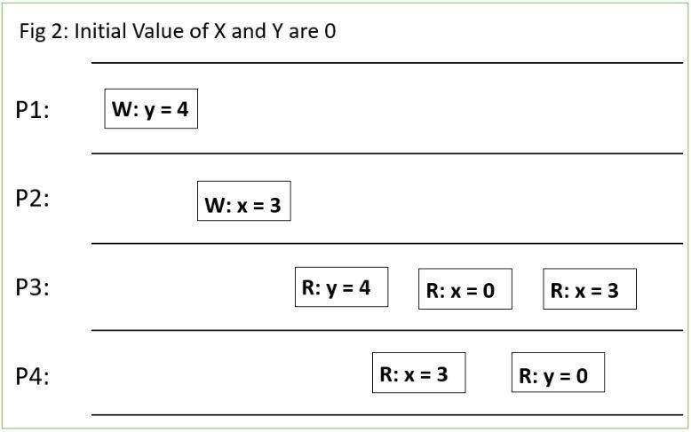
Here, P4 reads x as 3 but y as 0. But the write of y = 4 happened before the write of x = 3. Since P4 reads the write to x which happened at a time after y = 4 but failed to read the write of y = 4, Fig 2 is not sequentially consistent.

Strict Consistency

Theoretically, Strict consistency is the highest level of consistency that can be obtained by the system. 

It essentially means that all nodes in the system must see the latest update made to a record in any of the replicated nodes. Thus, if an update completes for a record in one node, anyone looking at that record from any of its replicated nodes should also see the latest update. 

The below Fig 3 illustrates the same.

It is mostly a theoretical concept as it is impossible to achieve in practice. This is because it stipulates that all nodes in the system agree on the current time and thus, the update as it is seen in one node is visible in another node at the same time. However, even multi-processor systems have some lag in aligning on the precise current time; let alone different nodes in a distributed system. 

Since Fig 3 is strictly consistent, it is also sequentially, causally, linearly and eventually consistent.

In contrast, Fig 1 and 2 were not strictly consistent.

Linearizable Consistency

In practice, this is the highest level of consistency that can be obtained in a distributed system. 

Linearizable Consistency has all the traits of Strict Consistency except that it accepts that a finite amount of time elapses before the update in one node is visible in another node.

The below Fig 4 shows this effect.

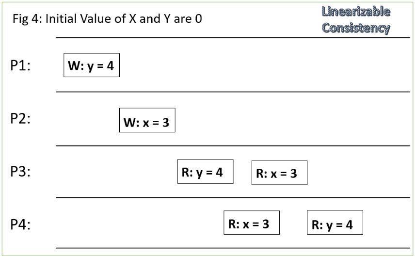
Since Fig 4 is linearly consistent, it is also sequentially, causally and eventually consistent.

In contrast, Fig 1 and 2 are not linearly consistent.

When we say that a system is consistent (Atomic Consistency) based on the CAP theorem, we mean that it is Linearly Consistent.

Causal Consistency

Causal Consistency is just below Sequential Consistency. 

The difference is that Causal Consistency does not enforce global ordering of both related and unrelated writes like Sequential Consistency. Instead, it enforces ordering of only related writes.

Say, there are two variables x and y with initial values as zero. Consider a code snippet with variable update that has a condition such as “if x = 1, then update y = 3”. Here, the update of y is related to the value of x. This makes it a related write.

Causal Consistency says that if any node has read x = 1 and then updated y as 3; then any node that reads x and y subsequently and reads y = 3 can do so only if it also reads x = 1. On the other hand, if a node reads x=0, then the value read as y can only be 0 and not 3.

Fig 5 illustrates this.

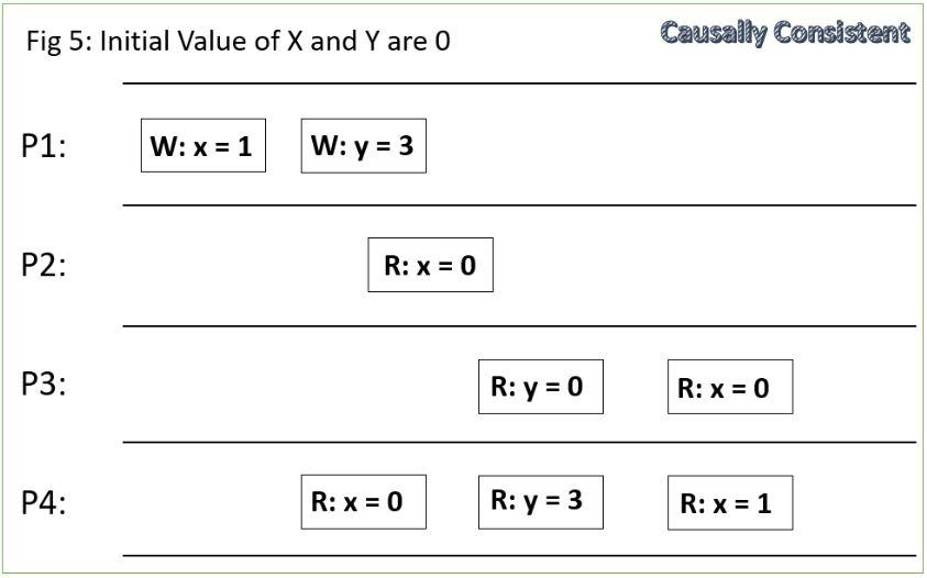
Since Fig 5 is Causally Consistent, it is also Eventually Consistent.

Eventual Consistency

Eventual Consistency is the weakest of this bunch. It just means that the system will be consistent – eventually.

I.e. an update that occurred in any of the nodes will also get updated in the other nodes eventually. The term ‘eventual’ is relative in terms of the time it takes to update all systems. It depends on how the Architect defines the time lag.

We can say that the distributed system will go about all its other activities without waiting for any consistency condition as they will not be enforced in an Eventually Consistent system.

The only guarantee in an Eventually Consistent system is that if there are no writes for a long period of time, then all nodes will agree on the last value. The ‘long’ is as defined by the Architect based on system requirements

Consider Fig 6 below:

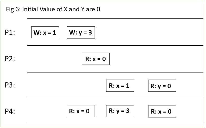
This system does not satisfy any other Consistency levels mentioned above. Eventual Consistency says that it might become consistent at a future point in time provided that there are no updates for a ‘long’ time.

ACID vs. BASE Systems

Perhaps obvious by now, ACID is a highly Consistent system whereas BASE is a highly Available system. 

Here, we can see that while the Consistency mentioned in the ACID semantics look different from that mentioned in the BASE or CAP theorem, it is in fact, a super set of Consistency requirements. What I mean by that is that the Consistency mentioned in CAP theorem is already implicit in ACID systems. 

To summarize, Consistency in ACID is stricter than the one in BASE. BASE has higher Availability than ACID.

References:

1) OLTP vs OLAP by IBM

2) ACID-BASE Consistency Models Explained